L1 & L2 regularization — Adding penalties to the loss function
Step by step implementation in Python
Regularization techniques are used to prevent overfitting in Neural Networks. Overfitting means learning the pattern and not generalizing it. We will look more into Overfitting when we will see Batch training.
In this post, we will implement L1 and L2 regularization in the loss function. In this technique, we add a penalty to the loss.
The L1 penalty means we add the absolute value of a parameter to the loss multiplied by a scalar.
And, the L2 penalty means we add the square of the parameter to the loss multiplied by a scalar.
How they are added to the loss and how they affect gradients will be discussed in this post.
You can download the Jupyter Notebook from here.
Note — This post uses many things from the previous chapters. It is recommended that you have a look at the previous posts.
5.3 L1 & L2 Regularization
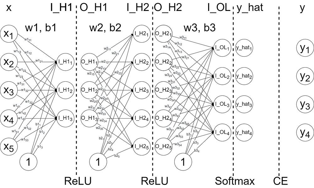
Note — The architecture of the Neural Network is the same as it was in the previous post, i.e., 4 layers with 5, 3, 5, and 4 nodes.
First, the activation function for the hidden layers is the ReLU function
Second, the activation function for the output layer is the Softmax function.
Third, the loss function used is Categorical cross-entropy loss, CE
Fourth, We will use SGD with Nesterov acceleration Optimizer with a learning rate = 0.01 and momentum = 0.9

Now, let us have a look at the steps.
Step 1 - A forward feed like we did in the previous post but with
         penalties included in loss
Step 2 - Initializing SGD with Nesterov acceleration Optimizer
Step 3 - Entering the training loop
      Step 3.1 - A forward feed to see loss with penalties before
                 training
      Step 3.2 - Using Backpropagation to calculate gradients
      Step 3.3 - Using SGD with Nesterov acceleration Optimizer to
                 update weights and biases
Step 4 - A forward feed to verify that the loss has been reduced
         and to see how close predicted values are to true values
Step 1 — A forward feed with penalties added to the loss
import numpy as np                          # importing NumPy
np.random.seed(42)input_nodes = 5                             # nodes in each layer
hidden_1_nodes = 3
hidden_2_nodes = 5
output_nodes = 4

x = np.random.randint(1, 100, size = (input_nodes, 1)) / 100
x                                       # Inputsy = np.array([[0], [1], [0], [0]])
y                                       # Outputs

def relu(x, leak = 0):                          # ReLU
    return np.where(x <= 0, leak * x, x)def relu_dash(x, leak = 0):                     # ReLU derivative
    return np.where(x <= 0, leak, 1)def softmax(x):                                 # Softmax
    return np.exp(x) / np.sum(np.exp(x))def softmax_dash(x):                            # Softmax derivative

    I = np.eye(x.shape[0])

    return softmax(x) * (I - softmax(x).T)def cross_E(y_true, y_pred):                    # CE
    return -np.sum(y_true * np.log(y_pred + 10**-100))def cross_E_grad(y_true, y_pred):               # CE derivative
    return -y_true/(y_pred + 10**-100)

w1 = np.random.random(size = (hidden_1_nodes, input_nodes))    # w1
b1 = np.zeros(shape = (hidden_1_nodes, 1))                     # b1w2 = np.random.random(size = (hidden_2_nodes, hidden_1_nodes)) # w2
b2 = np.zeros(shape = (hidden_2_nodes, 1))                     # b2w3 = np.random.random(size = (output_nodes, hidden_2_nodes))   # w3
b3 = np.zeros(shape = (output_nodes, 1))                       # b3

Now, before calculating loss we will add penalties.
- We will add L1 and L2 penalties on weights w3 and biases b3 with regularization value L1 = 0.01 and L2 = 0.01
- We will add L1 penalty on weights w2 and biases b2 with regularization vale L1 = 0.01
- We will add L2 penalty on weights w1 and biases b1 with regularization vale L2 = 0.01
Note — You will find in many references that L1 and L2 regularization is not used on biases, but to show you how easy it is to implement, we will do it here. And you can use different regularization values for different parameters if you want.
l1 = 0.01 # L1 regularization valuel2 = 0.01 # L2 regularization value

Let us see how to add penalties to the loss.
When we say we are adding penalties, we mean this

Or, in reduced form for Python, we can do this.

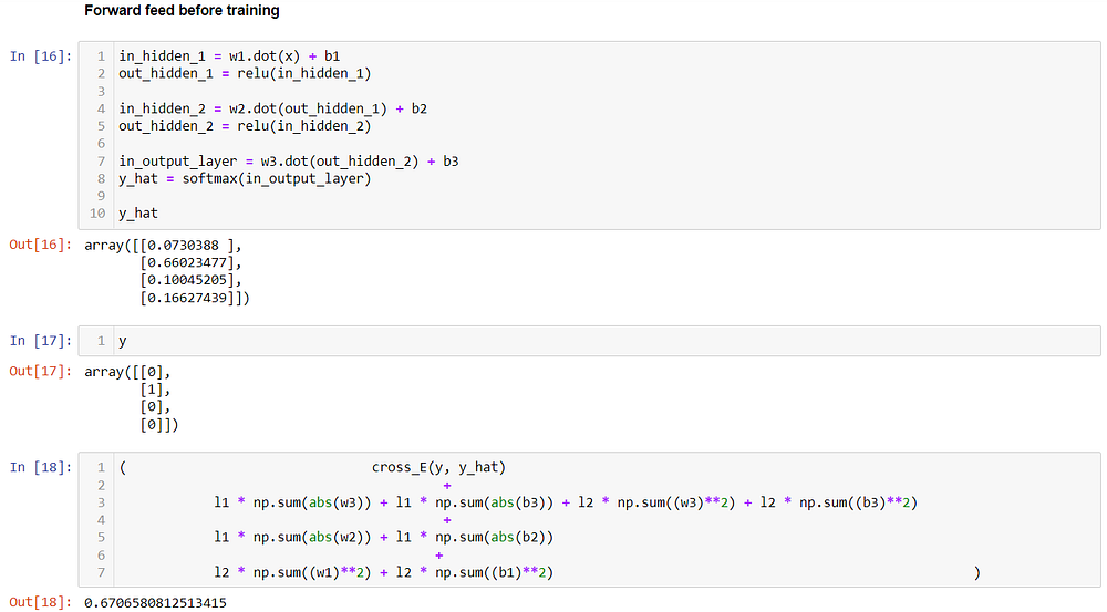
The forward feed will look like this,
in_hidden_1 = w1.dot(x) + b1                   # forward feed
out_hidden_1 = relu(in_hidden_1)in_hidden_2 = w2.dot(out_hidden_1) + b2
out_hidden_2 = relu(in_hidden_2)in_output_layer = w3.dot(out_hidden_2) + b3
y_hat = softmax(in_output_layer)y_hat                                          # y_haty                                              # y(                      cross_E(y, y_hat)       # loss with penalties
                               +
            l1 * np.sum(abs(w3)) + l1 * np.sum(abs(b3))
            + l2 * np.sum((w3)**2) + l2 * np.sum((b3)**2)
                               +
            l1 * np.sum(abs(w2)) + l1 * np.sum(abs(b2))
                               +
            l2 * np.sum((w1)**2) + l2 * np.sum((b1)**2)            )

Step 2 — Initializing SGD with Nesterov acceleration Optimizer
learning_rate = 0.01 # learning ratemomentum = 0.9 # momentumupdate_w1 = np.zeros(w1.shape) # Initializing updates with 0update_b1 = np.zeros(b1.shape)update_w2 = np.zeros(w2.shape)update_b2 = np.zeros(b2.shape)update_w3 = np.zeros(w3.shape)update_b3 = np.zeros(b3.shape)

Step 3 — Entering training loop
epochs = 1000
Step 3.1 — A forward feed to see loss before training
We will print loss before training every time to see that it is reducing after each training epoch.
for epoch in range(epochs):#---------------------Forward Propagation---------------------------

    in_hidden_1 = w1.dot(x) + b1
    out_hidden_1 = relu(in_hidden_1)    in_hidden_2 = w2.dot(out_hidden_1) + b2
    out_hidden_2 = relu(in_hidden_2)    in_output_layer = w3.dot(out_hidden_2) + b3
    y_hat = softmax(in_output_layer)

    loss = (               cross_E(y, y_hat)
                                  +
                  l1 * np.sum(abs(w3)) + l1 * np.sum(abs(b3))
                 + l2 * np.sum((w3)**2) + l2 * np.sum((b3)**2)
                                  +
                  l1 * np.sum(abs(w2)) + l1 * np.sum(abs(b2))
                                   +
                  l2 * np.sum((w1)**2) + l2 * np.sum((b1)**2)      )

    print(f'loss before training is {loss} -- epoch number {epoch +
                                                                1}')
    print('\n')

Step 3.2 — Calculating gradients via Backpropagation
Here is the answer to your question. How gradients are affected by penalties in the loss?
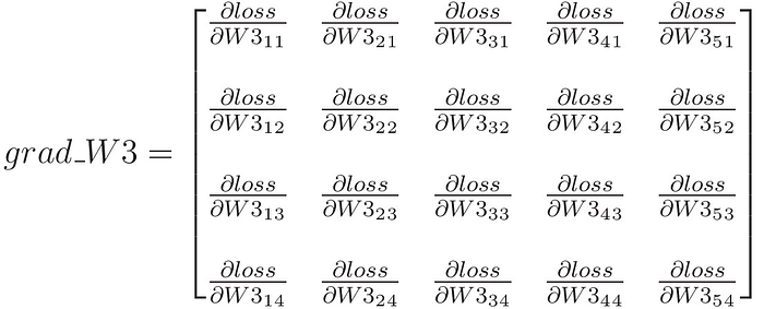
If you remember from the last post, we need to calculate grad_w3 which is

Let us take the first term, i.e.,

From the loss term, we can see that

So, like this, for every term in grad_w3, we can write this

or,

We already know how to calculate the first matrix.
And the second and the third matrix can be reduced to

Like this, we cal calculate gradients for b3, w2, b2, w1, and b1. All we have to do is add the reduced form of penalty derivatives in the gradients.
So, now let us take a look at the gradients in Python
#--------------Gradient Calculations via Back Propagation-----------    error_upto_softmax = np.sum(cross_E_grad(y, y_hat) *
           softmax_dash(in_output_layer), axis = 0).reshape((-1, 1))

    grad_w3 = error_upto_softmax .dot( out_hidden_2.T ) + l1 * (w3 /
                                 (abs(w3) + 10**-100)) + l2 * 2 * w3

    grad_b3 = error_upto_softmax + l1 * (b3 / (abs(b3) + 10**-100))
                                                       + l2 * 2 * b3

    #-----------------------------------------

    error_grad_H2 = np.sum(error_upto_softmax * w3, axis = 0)
                                                   .reshape((-1, 1))

    grad_w2 = error_grad_H2 * relu_dash(in_hidden_2) .dot(
                 out_hidden_1.T ) + l1 * (w2 / (abs(w2) + 10**-100))

    grad_b2 = error_grad_H2 * relu_dash(in_hidden_2) + l1 * (b2 /
                                               (abs(b2) +10**-100))

    #-----------------------------------------

    error_grad_H1 = np.sum(error_grad_H2 * relu_dash(in_hidden_2) *
                                     w2, axis = 0) .reshape((-1, 1))

    grad_w1 = error_grad_H1 * relu_dash(in_hidden_1) .dot( x.T ) +
                                                         l2 * 2 * w1

    grad_b1 = error_grad_H1 * relu_dash(in_hidden_1) + l2 * 2 * b1

Step 3.3 — Using SGD with Nesterov acceleration Optimizer to update the weights and biases
#--------Updating weights and biases with SGD Momentum Nesterov-----    update_w1 = - learning_rate * grad_w1 + momentum * update_w1
    update_w1_ = - learning_rate * grad_w1 + momentum * update_w1
    w1 += update_w1_                                  # w1

    update_b1 = - learning_rate * grad_b1 + momentum * update_b1
    update_b1_ = - learning_rate * grad_b1 + momentum * update_b1
    b1 += update_b1_                                  # b1

    update_w2 = - learning_rate * grad_w2 + momentum * update_w2
    update_w2_ = - learning_rate * grad_w2 + momentum * update_w2
    w2 += update_w2_                                  # w2

    update_b2 = - learning_rate * grad_b2 + momentum * update_b2
    update_b2_ = - learning_rate * grad_b2 + momentum * update_b2
    b2 += update_b2_                                  # b2

    update_w3 = - learning_rate * grad_w3 + momentum * update_w3
    update_w3_ = - learning_rate * grad_w3 + momentum * update_w3
    w3 += update_w3_                                  # w3

    update_b3 = - learning_rate * grad_b3 + momentum * update_b3
    update_b3_ = - learning_rate * grad_b3 + momentum * update_b3
    b3 += update_b3_                                  # b3

The training loop will run 1,000 times.

This is a small screenshot after the training.
Step 4 — A forward feed to verify that the loss is reduced and to see how close predicted values are to true values
in_hidden_1 = w1.dot(x) + b1                      # forward feed
out_hidden_1 = relu(in_hidden_1)in_hidden_2 = w2.dot(out_hidden_1) + b2
out_hidden_2 = relu(in_hidden_2)in_output_layer = w3.dot(out_hidden_2) + b3
y_hat = softmax(in_output_layer)y_hat                                             # predicted valuesy                                                 # true values(                      cross_E(y, y_hat)       # loss with penalties
                               +
            l1 * np.sum(abs(w3)) + l1 * np.sum(abs(b3))
            + l2 * np.sum((w3)**2) + l2 * np.sum((b3)**2)
                               +
            l1 * np.sum(abs(w2)) + l1 * np.sum(abs(b2))
                               +
            l2 * np.sum((w1)**2) + l2 * np.sum((b1)**2)            )

I hope now you understand how to implement L1 and L2 regularization in Neural Networks.
If you like this post then please subscribe to my youtube channel neuralthreads and join me on Reddit.
I will be uploading new interactive videos soon on the youtube channel. And I will be happy to help you with any doubt on Reddit.


